🔎📊 Principal Component Analysis with XGBoost Regression in Python

Summary-

This project is based on data from the Mercedes Benz test bench for vehicles at the testing and quality assurance phase during the production cycle. The dataset consists of high number of feature columns. Key highlights from the project include - Dimensionality reduction using PCA and XGBoost Regression used after the dimensionality reduction to predict the time required to test the vehicles

You can view the full project code on this Github link

Note: This is an academic project completed by me as part of my Post Graduate program in Data Science from Purdue University through Simplilearn. The project was towards the completion of Data Science Machine Learning module.

Bussiness Scenario

Since the first automobile, the Benz Patent Motor Car in 1886, Mercedes-Benz has stood for important automotive innovations. These include the passenger safety cell with a crumple zone, the airbag, and intelligent assistance systems. Mercedes-Benz applies for nearly 2000 patents per year, making the brand the European leader among premium carmakers. Mercedes-Benz is the leader in the premium car industry. With a huge selection of features and options, customers can choose the customized Mercedes-Benz of their dreams.
To ensure the safety and reliability of every unique car configuration before they hit the road, the company’s engineers have developed a robust testing system. As one of the world’s biggest manufacturers of premium cars, safety and efficiency are paramount on Mercedes-Benz’s production lines. However, optimizing the speed of their testing system for many possible feature combinations is complex and time-consuming without a powerful algorithmic approach.
We are required to reduce the time that cars spend on the test bench. Then we will work with a dataset representing different permutations of features in a Mercedes-Benz car to predict the time it takes to pass testing. Optimal algorithms will contribute to faster testing, resulting in lower carbon dioxide emissions without reducing Mercedes-Benz’s standards.

Objective

Reduce the time a Mercedes-Benz spends on the test bench.

Analysis Steps

1. Load the data :
   • Load the train and test data csv files.
   • Print first few rows of this data using head function.
   • Review the shape of the data(i.e. No. of rows = Samples and No. of Columns = Features).
     Initially we notice the data consists of 377 feature columns.
2. Data Cleaning :
   • Check for any column(s),if the variance is equal to zero, then we can remove those variable(s)/feature(s). This can be done by reviewing if for any column the number of unique values is equal to 1. Then those columns are constant for all the samples in the data and would not have any impact in the prediction of the target variable ‘y’
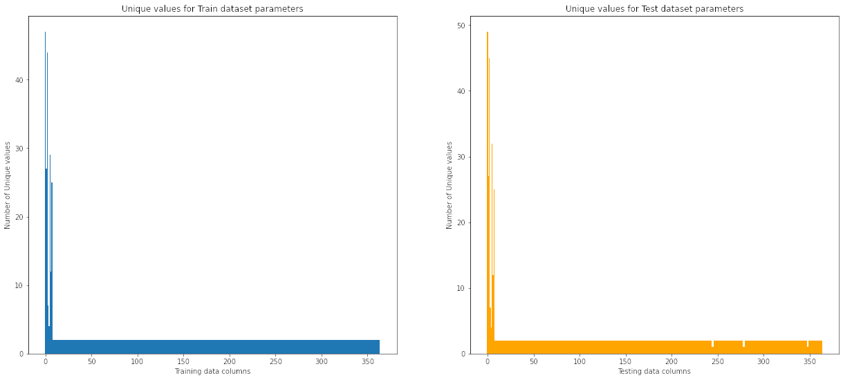
   • Check for null values and unique values for both the train and test data.
     After removing the columns with no variance we are left with 365 columns/features from the original data.

   

3. Data Pre-processing :
   There are some columns in the data set which are categorical. For performing PCA these need to be encoded to numerical form. We first find the relevant columns, then proceed to apply label encoding as some of these columns have many unique values which would make one-hot encoding undesirable for this problem as it would generate too many dummy variables.

4. Dimensionality Reduction :
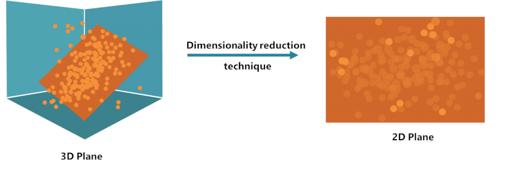
   For dimensionality reduction we will use the Principal Component Analysis technique. Principal Component Analysis (PCA) is a statistical procedure that uses an orthogonal transformation that converts a set of correlated variables to a set of uncorrelated variables. PCA is the most widely used tool in exploratory data analysis and in machine learning for predictive models. Moreover, PCA is an unsupervised statistical technique used to examine the interrelations among a set of variables.

   

   We use PCA implementation which is part of the sklearn decomposition package.
   Note: Before we apply PCA transformation for the data. We need to ensure the data is standardized. Hence we first apply the Standard scaling for the Train and test data and then proceed to apply the PCA transformation.
   Also PCA transformation by itself does not reduce the number of components. PCA actually expresses all the features/variables in the original data-set as principal components (linear combinations of original features based on the eigen decomposition). We can then select the number of such principal components to reduce the number of dimensions when building models or analysing the data further. Under PCA one can directly specify the number of components you want to extract OR we can mention the minimum amount of the variance of the original data which must be explained by the components.
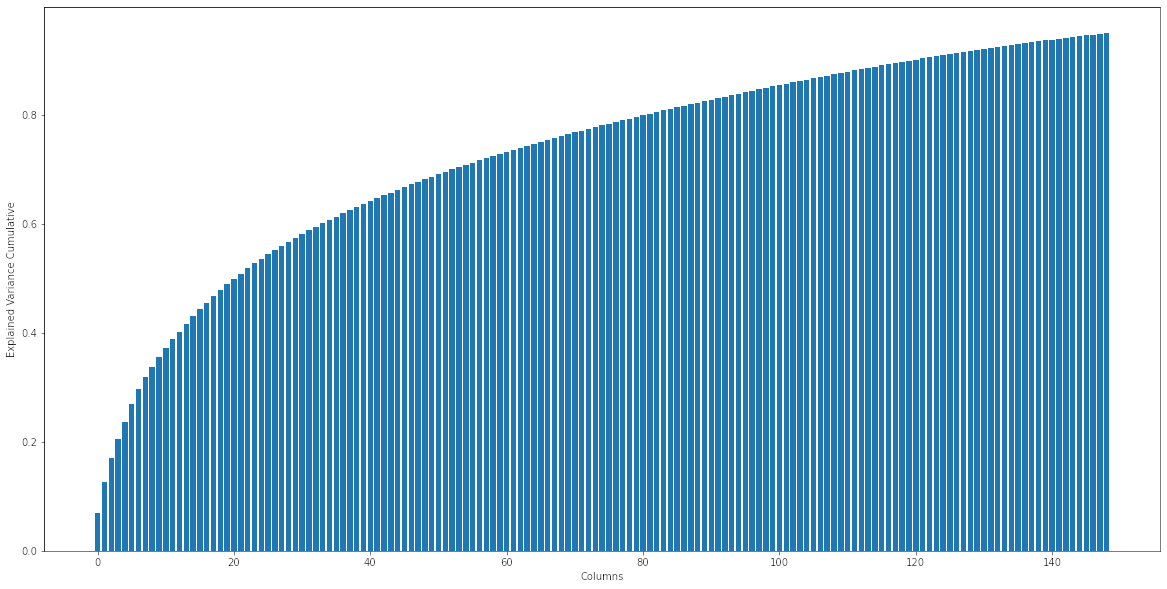
   In this case we want to select the reduced number of components such that 95% of the original data variance is explained by the selected principal components. So when applying PCA transformation we set the n_components value to 0.95.

   

   After running the transformation we see that 149 principal components account for 95% of the information/variance from the original dataset.

5. Model Building :
   Build a regression model on the data using XGBoost algorithm using the reduced/transformed version of the data after PCA with reduced features(principal components). The objective is to predict target variable ‘y’ which is the time taken to test the vehicles(i.e. time spent by the vehicle on the test bench).
   • For the XGBoost Regressor we first try to find the best parameters on the Train data using GridSearchCV method.
   • Next we have done K-fold cross validation using the best parameters model obtained by previous step.
   • Finally we fit the model on the train data and check the overall accuracy. Then predict ‘y’ using the model on the test data. Note that since test data did not have the ‘y’ label. We cannot verify the accuracy of the model on the test data.
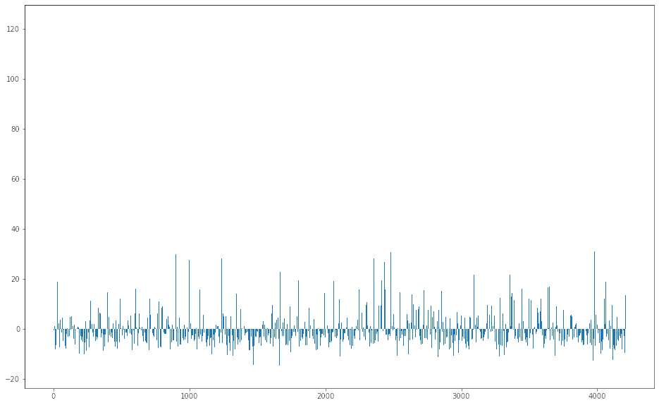
   • Since we cannot verify the accuracy on test data, we have reviewed the model accuracy on the train data. Reviewed the actual v/s predicted values and same was plotted to visualize the quantity of deviation(error) from the actual y values.

   

Tools used:

This project was completed in Python using Jupyter notebooks. Common libraries used for analysis include numpy, pandas, matplotlib, sklearn and xgboost