
Summary-
This is comprehensive project completed by me as part of the Data Science Post Graduate Programme.
This project includes multiple classification algorithms over a dataset collected on health/diagnostic variables to predict of a person has diabetes or not based on the data points. Apart from extensive EDA to understand the distribution and other aspects of the data, pre-processing was done to identify data which was missing or did not make sense within certain columns and imputation techniques were deployed to treat missing values. For classification the balance of classes was also reviewed and treated using SMOTE.
Finally models were built using various classification algorithms and compared for accuracy on various metrics.Lastly the project contains a dashboard on the original data using Tableau.
You can view the full project code on this Github link
Note: This is an academic project completed by me as part of my Post Graduate program in Data Science from Purdue University through Simplilearn. This project was towards final course completion.
Bussiness Scenario
This dataset is originally from the National Institute of Diabetes and Digestive and Kidney Diseases. The objective of the dataset is to diagnostically predict whether or not a patient has diabetes, based on certain diagnostic measurements included in the dataset. Several constraints were placed on the selection of these instances from a larger database. In particular, all patients here are females at least 21 years old of Pima Indian heritage.
Objective
Build a model to accurately predict whether the patients in the dataset have diabetes or not.
Analysis Steps
Data Cleaning and Exploratory Data Analysis -
- Perform descriptive analysis. It is very important to understand the variables and corresponding values.
- Can minimum value of below listed columns be zero (0)? On these columns, a value of zero does not make sense and thus indicates missing value.
- Glucose
- BloodPressure
- SkinThickness
- Insulin
- BMI
In this section we load the data and use the describe function of pandas for dataframes to view the quick snapshot of the statistical measures. There are no Nan values in the 768 rows. However as mentioned before we analyse the listed columns for 0 values and note that there are missing i.e.(0) values in all the columns. But for 2 of the columns SkinThickness and Insulin there is a high proportion of missing values.
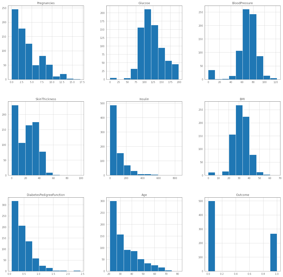
- Decide how to treat the zero values in these columns - For imputation we need to observe the distribution of the variables to identify if mean or median imputation would be appropriate.
- Visually explore these variables and look for the distribution of these variables using histograms. Treat the missing values accordingly.
![histogram]()
- We review the skewness of the distributions to decide if the imputation should be using mean or median. If the distribution has less skewness mean imputation can be done. For skewed data the median is more appropriate.
- Using the rule we have applied mean imputation only for BloodPressure. For the remaining 4 columns median imputation was done for the 0 values.
- Can minimum value of below listed columns be zero (0)? On these columns, a value of zero does not make sense and thus indicates missing value.
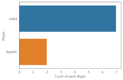
There are integer as well as float data-type of variables in this dataset. Create a count (frequency) plot describing the data types and the count of variables.
![count plot of data types]()
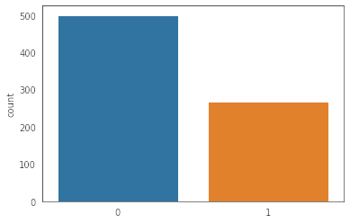
Check the balance of the data (to review imbalanced classes for the classification problem) by plotting the count of outcomes by their value. Review findings and plan future course of actions.
![class imbalance]()
We notice that there is class imbalance . The diabetic class (1) is the minority class and there are 35% samples for this class. However for the non-diabetic class(0) there are 65% of the total samples present. We need to balance the data using any oversampling for minority class or undersampling for majority class. This would help to ensure the model is balanced across both classes.We can apply the SMOTE (synthetic minority oversampling technique) method for balancing the samples by oversampling the minority class (class 1 - diabetic) as we would want to ensure model more accurately predicts when an individual has diabetes in our problem.
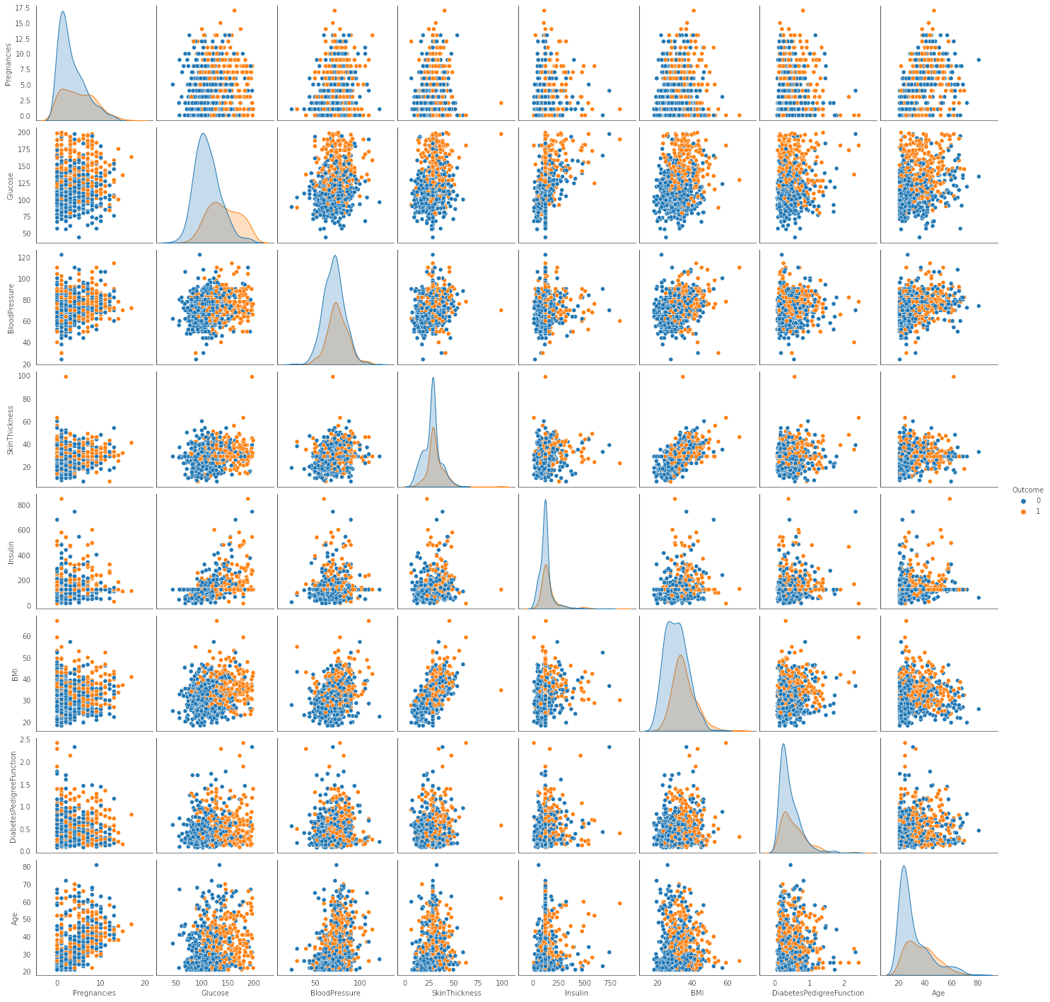
Create scatter charts between the pair of variables to understand the relationships. Describe findings.
![Pair plots]()
We review scatter charts for analysing inter-relations between the variables and observe the following
- Most features do not show any strong correlation or patterns from the scatter plots.
- Only the following feature-pairs (BMI and SkinThickness) and (Glucose and Insulin) show some level of positive correlation
- Class seperation(Diabetic vs non diabetic) looks better in pairs containing “Glucose” as a feature. This could imply that the feature would contribute more to the classification and be a significant part of the model.
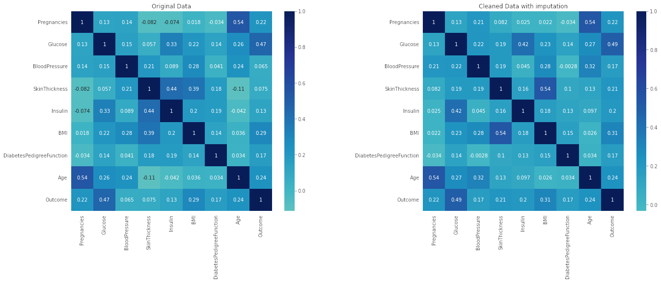
Perform correlation analysis. Visually explore it using a heat map.
![correlation matrix plots]()
Observation : As mentioned in the pairplot analysis the variable Glucose has the highest correlation to outcome.
- Perform descriptive analysis. It is very important to understand the variables and corresponding values.
Model Building
- Devise strategies for model building. It is important to decide the right validation framework. Would Cross validation be useful in this scenario?
- A. Guideline/Main Approach
For this problem, as it is true in the case of most other medical applications of classification algorithms we would want a model to ensure that we are able to correctly identify the cases where persons have the disease correctly. So based on this we concluded the worst case scenario to be a false negative.
🔴 False negative – A person we told is not diabetic, but is actually having diabetes This makes for a worse situation as we gave a false signal to a person who requires treatment. If left untreated or untested this may lead to more health complications and severe consequences So based on the framework for this problem our aim should be to have a model where we are able to reduce the false-negatives as much as possible making the recall-score(sensitivity a more important factor) when making decisions for model selection - B. Model building Strategy and Approach
We will follow the below steps in building and model selection for the problem :
- First we perform resampling using SMOTE so that the classes(diabetic - 1 and non-diabetic - 0) are balanced in the data.
- Next we will split the data into Train-test(validation) split. The split will be done with a stratified sampling method to ensure that the splits retain the class distribution or proportion of samples for both classes. This step is done first to ensure there is no data leakage on the following steps where we will test models again using the validation data-set to decide the optimum model.
- Before we proceed with the model building. We would need to ensure that data is scaled uniformly. We will perform standard scaling as a final pre-processing step to bring all the features to same scale which is advisable for applying distance based algorithms like KNN.
- Next we shall proceed with model building. First we will build a model on KNN algorithm as a baseline with the best value of n_neighbors through GridSearchCV.
- Next we can run the K-Fold cross validation using the training data for the various other models to be tested on the classification problem. This should give us a idea of the overall performance of the models on multiple samples picked randomly from the train data.
- Finally we can again test the models on the validation data to analyse the classification model(s) with the best possible accuracy and recall. Model scores will be compared with scores from the KNN alogrithm identified in step 4.
- Lastly the final model is selected based on the validation criteria (i.e. best accuracy and recall) on test data along with good results on the train data during k-fold cross validation . Model also needs to be evaluated using various other metrics like f-1 score, confusion matrix and classification summary with auc score(roc curve), sensitivity and specificity metrics
- A. Guideline/Main Approach
- Apply an appropriate classification algorithm to build a model. Compare various models with the results from KNN.
- For KNN model the best value of n_neigbors = 17 based on GridSearch_CV which resulted in best combined score (i.e. best accuracy and recall scores).
- Random Forest Model has the best Combined score on Validation(test) data and this result is consistent with the results from K-fold cross validation on train data. XGBoost was second best on combined score, although we see XGB actually has better recall but Random forest had better accuracy overall leading to the slightly better combined score.
- The next 2 best performing models were SVM which is 4th on the and KNN has the 3rd best combined score on the (test)validation data due to it getting better recall than SVM.
- So overall we can see that Random forest gives us the best mix of accuracy with recall.
- We will shortlist the following 3 models Random Forest, XGBoost and K-Nearest Neighbors Classifier for the next step of analysis before we finalize the optimal model.
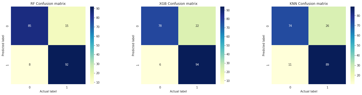
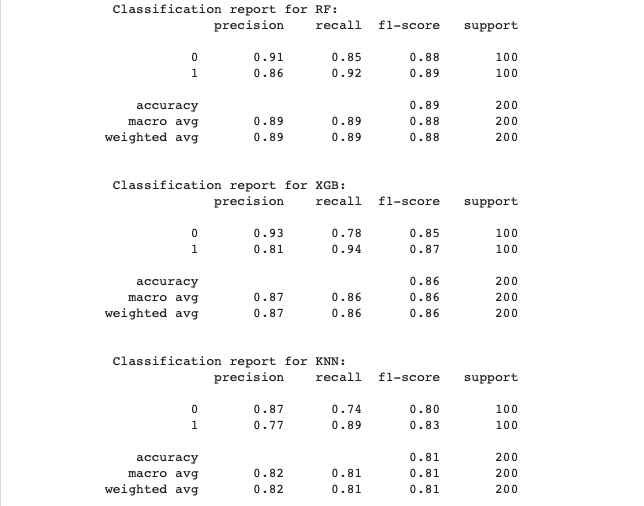
Create a classification report by analysing sensitivity, specificity, AUC(ROC curve) etc. Decide what values of these parameter to settle for? any why?
![Confusion Matrix]()
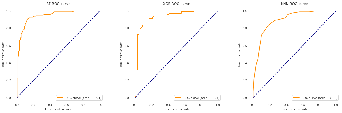
![AUC ROC Curve]()
![Classification Report]()
We tested the models using confusion matrix, classification report and finally AUC(ROC) curve.Model AUC Sensitivity Specificity RF 94.260 92.0 85.0 XGB 93.010 94.0 78.0 KNN 89.555 89.0 74.0 Note: ROC (Receiver Operating Characteristic) Curve tells us about how good the model can distinguish between two things (e.g If a patient has a disease or no). Better models can accurately distinguish between the two. Whereas, a poor model will have difficulties in distinguishing between the two. This is quantified in the AUC Score. Final Analysis Based on the classification report:
- As per the framework decided earlier the sensitivity score is important and we can consider 90% as a minimum benchmark.
- Once again we see as per the classification report, AUC score is best for Random forest model. This means the model is able to differentiate the best between the two classes in the data. And while it has a lower sensitivity score than XGB model. It has a much better specificity score. Further note that the sensitivity score is not significantly lower for Random Forest when compared to XGBoost model. Both models clear the benchmark level of 90% on sensitivity.
- KNN scored lower than both Random Forest and XGBoost model overall.
Based on these metrics we can select Random forest model to be the optimal model for this problem.
- Devise strategies for model building. It is important to decide the right validation framework. Would Cross validation be useful in this scenario?
Data Reporting
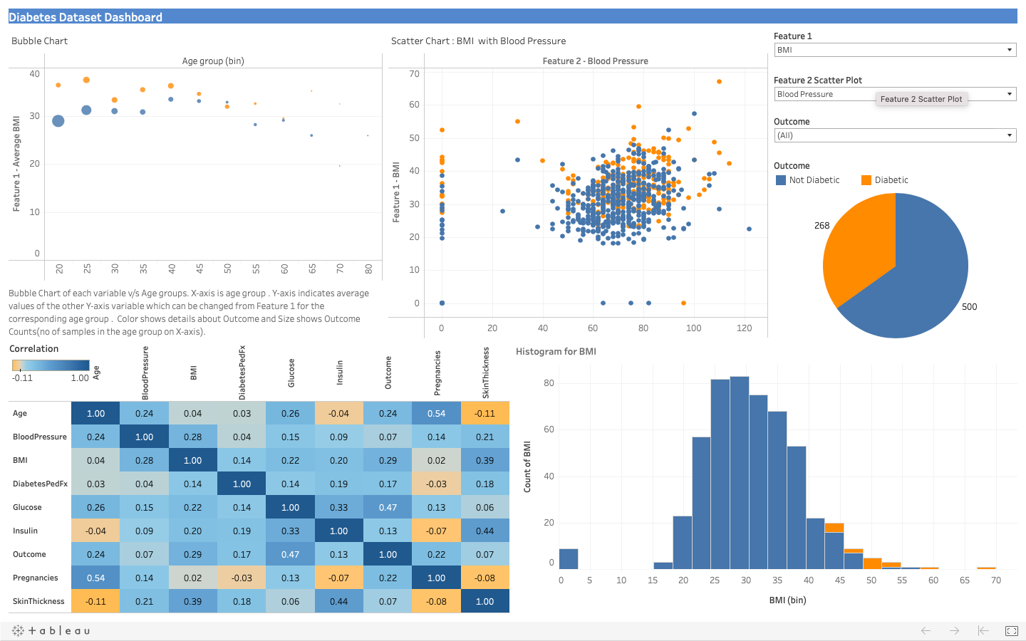
- Dashboard in tableau by choosing appropriate chart types and metrics useful for the business. The dashboard must entail the following:
- Pie chart to describe the diabetic/non-diabetic population
- Scatter charts between relevant variables to analyse the relationships
- Histogram/frequency charts to analyse the distribution of the data
- Heatmap of correlation analysis among the relevant variables
- Create bins of Age values – 20-25, 25-30, 30-35 etc. and analyse different variables for these age brackets using a bubble chart.
To view the tableau visualization visit this Tableau public page link
![Dashboard Tableau]()
- Dashboard in tableau by choosing appropriate chart types and metrics useful for the business. The dashboard must entail the following:
Tools used:
This project was completed in Python using Jupyter notebooks. Common libraries used for analysis include numpy, pandas, sci-kit learn, matplotlib, seaborn, xgboost